Optimization: Linear Programming

Purpose

This calculator solves a linear programming problem that you define yourself — you choose the optimization direction, name your own decision variables, write your own objective function, and enter your own constraints as plain math expressions.

Unlike the other Optima calculators, which already come with a fixed table structure for a named business problem, this one puts you in the driver's seat. It answers a very direct question: given whatever variables and constraints you can express in ordinary algebra, what values of those variables make the objective as large (or as small) as possible without breaking any of the rules you wrote?

Background

Problem Domain

Linear programming is the foundation nearly every other calculator in the Optima family is built on — transportation, blending, capacity, and the rest are all linear (or mixed-integer) programs with a fixed shape, wrapped in a friendlier table interface. This calculator strips that wrapper away and exposes the raw solver directly, so you can model a problem that doesn't fit any of the ready-made templates.

Real-World Uses

• One-off decision problems: Your situation doesn't match any named Optima calculator (transport, blending, capacity, and so on). Use this model to describe the exact variables, objective, and constraints for your specific case without waiting for a dedicated calculator.
• Learning and teaching linear programming: Textbook and coursework problems are usually already written as an objective function plus a list of constraints. Use this calculator to type them in directly and see the optimal solution, without translating them into a specialized template.
• Quick feasibility or boundedness checks: Before investing time building a full table-driven model, you want to know whether a small set of constraints is even feasible, or whether the objective is unbounded. Use this calculator to test that in a couple of minutes.
• Two-variable trade-off exploration: With exactly two decision variables, the result includes a feasible-region chart. Use this calculator to see the geometry of a small trade-off problem — which corner of the feasible region the optimum sits at, and why.

Inputs

• objective: Optimization direction. Choose Maximize or Minimize for objective_function.
• decision_variables: List of decision variable definitions, one entry per variable, for example x >= 0 or y >= 0. Each entry names one variable and optionally sets a single bound:
• a bare name defaults to a lower bound of 0 (the usual non-negativity assumption).
• name >= number sets a lower bound.
• name <= number sets an upper bound. Every variable used in objective_function or constraints must be declared here.
• objective_function: The expression to maximize or minimize, written using the declared variable names, for example 3*x + 5*y. Multiplication must be written explicitly with * (for example 3*x, not 3x).
• constraints: List of constraint expressions, one entry per constraint, for example 2*x + 3*y >= 12. Each entry must have all variable terms on the left-hand side and a single numeric constant on the right-hand side, joined by <=, >=, or =.

Results

• Status: Solver outcome such as Optimal, Infeasible, Unbounded, Not Solved, or Undefined. This is the first thing to check — only an Optimal status means the other values represent a genuine best answer.
• Status Description: A plain-language explanation of Status, for example confirming a finite optimal solution was found or that no solution satisfies every constraint.
• Objective: The optimized value of objective_function at the solution. This is the best achievable value given every constraint you entered.
• One result per declared decision variable, named after the variable itself (for example x, y): its optimal value at the solution. Together, these values are the actionable answer — the specific quantities that achieve the reported Objective.
• chart (only when there are exactly two decision variables and the status is Optimal): A feasible-region chart plotting the constraints, the feasible area, and the optimal point. This gives a visual explanation of why that particular corner of the feasible region is the best one.

Understanding the Calculation

Every decision variable, the objective, and every constraint are parsed as ordinary algebraic expressions and handed to a linear programming solver, which finds the corner of the feasible region — the intersection of all your constraints and variable bounds — that gives the best objective value. This is the same simplex-family approach used by every other Optima calculator; here it is exposed directly instead of being wrapped in a fixed table.

Example

Example courtesy of J E Beasley, people.brunel.ac.uk (OR-Notes, "Linear programming example 1997 UG exam").

A company makes two products, X and Y, on two machines, A and B. Each unit of X takes 50 minutes on machine A and 30 minutes on machine B; each unit of Y takes 24 minutes on machine A and 33 minutes on machine B. At the start of the week there are already 30 units of X and 90 units of Y in stock. Machine A has 40 hours available this week and machine B has 35 hours. Demand for the week is forecast at 75 units of X and 95 units of Y, and company policy is to maximize the combined stock of X and Y left over at the end of the week.

Let x be the number of units of X produced this week and y the number of units of Y produced this week. Ending stock is (x + 30 - 75) for X and (y + 90 - 95) for Y, so the quantity to maximize is (x + 30 - 75) + (y + 90 - 95), which simplifies to x + y - 50. Production must cover demand net of existing stock, giving x >= 75 - 30 = 45 and y >= 95 - 90 = 5. Machine time gives the two remaining constraints, converting hours to minutes: 50*x + 24*y <= 40*60 = 2400 and 30*x + 33*y <= 35*60 = 2100.

This maps directly onto the calculator's inputs:

• objective: Maximize
• decision_variables: x >= 45, y >= 5
• objective_function: x + y - 50
• constraints: 50*x + 24*y <= 2400, 30*x + 33*y <= 2100

Solving gives Status: Optimal with x = 45, y = 6.25, and Objective = 1.25. Because there are exactly two variables, the result also includes a feasible-region chart.

Interpretation

The solver keeps x pinned at its minimum of 45 — producing any more X than demand requires only eats into machine time without helping the objective, since X earns no more "stock benefit" per unit than Y does.

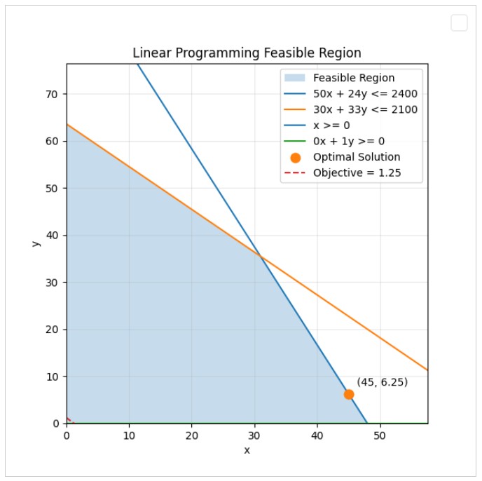
Fig: Liner programming example

Machine A's time is fully used at that point (50*45 + 24*6.25 = 2400), which is exactly why the source material calls this a graphical intersection of x = 45 and 50x + 24y = 2400 — the optimum sits precisely where the production-minimum boundary meets the busiest machine's limit, with only 1.25 combined units left over as spare stock at week's end.

Important Assumptions and Limitations

• All relationships are linear: squared terms, products of two variables, or other nonlinear expressions are not supported in objective_function or constraints.
• Decision variables are treated as continuous by this calculator; there is no option here for integer or binary variables. Use one of the dedicated Optima calculators (such as Knapsack, Assignment, or Supplier Selection) when whole-number or yes/no decisions matter.
• Each variable should be declared exactly once in decision_variables. If the same name appears more than once, only the last definition is kept and earlier bounds are silently discarded — combining both a lower and an upper bound for one variable through this list is not supported.
• Each constraint's right-hand side must be a plain number, not an expression or another variable; move all variable terms to the left-hand side first.
• The feasible-region chart is produced only for problems with exactly two decision variables and an Optimal status.